Mastering Frontal Plane Malalignment: The Paley Malalignment Test
Key Takeaway
Dr. Paley's Malalignment Test systematically evaluates lower extremity frontal plane deformities. It uses radiographic measurements (mLDFA, MPTA, Joint Line Convergence) to pinpoint anatomical sources of Mechanical Axis Deviation. This guides precise osteotomies, restoring joint biomechanics.
Frontal Plane Malalignment and Malorientation
The evaluation and correction of lower extremity deformities have been fundamentally transformed by the principles established by Dr. Dror Paley. Moving away from subjective, visual estimation, modern orthopedic deformity correction relies on a rigorous, geometric, and biomechanical approach. Understanding malalignment and malorientation in the frontal plane is the cornerstone of this methodology.
For orthopedic surgeons, residents, and fellows, mastering these concepts is not merely an academic exercise; it is an absolute prerequisite for executing precise osteotomies, restoring normal joint biomechanics, and preventing premature joint degeneration. This comprehensive guide dissects the frontal plane analysis, focusing on the Malalignment Test, the identification of deformity sources, and the application of Paley Center of Rotation of Angulation principles.
Principles of Deformity Correction
The primary goal of lower extremity deformity correction is to restore the mechanical axis of the limb, ensuring that ground reaction forces pass appropriately through the center of the hip, knee, and ankle joints. When the mechanical axis deviates from its normal trajectory, the resulting asymmetrical load distribution accelerates cartilage wear, stretches ligamentous structures, and ultimately leads to osteoarthritis.
Dr. Paley’s approach emphasizes the distinction between alignment and orientation:
* Alignment refers to the collinearity of the centers of the hip, knee, and ankle joints.
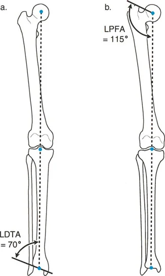
* Orientation refers to the angle at which the joint lines intersect the mechanical or anatomic axes of the respective long bones.
A limb can be perfectly aligned (normal mechanical axis) but severely maloriented (abnormal joint angles), which still results in pathological joint shear forces. Conversely, a limb can be malaligned but have normal joint orientation if the deformity is purely diaphyseal and compensated.
Understanding Mechanical Axis Deviation
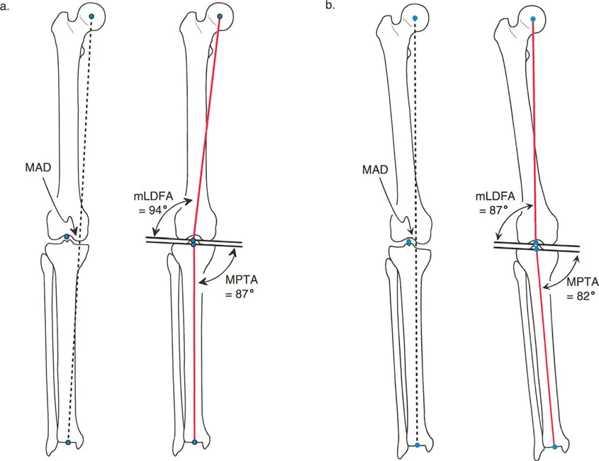
Mechanical Axis Deviation is the absolute measurement of frontal plane malalignment. It quantifies the distance by which the mechanical axis of the lower extremity misses the center of the knee joint.
In a normal, healthy lower extremity, the mechanical axis line drawn from the center of the femoral head to the center of the tibial plafond passes slightly medial to the exact center of the knee joint. The normal physiological Mechanical Axis Deviation is 8 ± 7 mm medial. Any deviation outside this physiological range indicates a pathological malalignment that warrants systematic investigation to identify its anatomical source.
The Malalignment Test
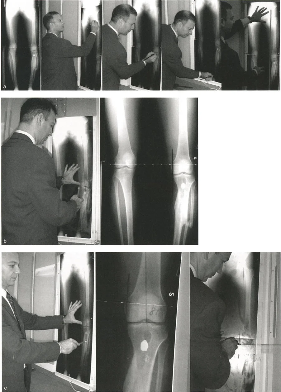
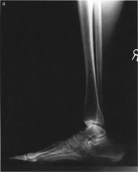
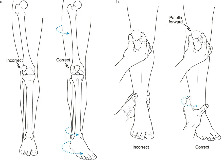
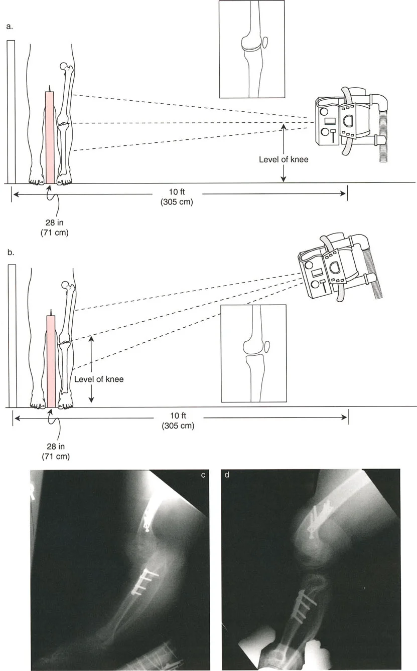
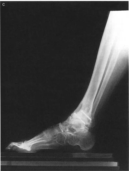
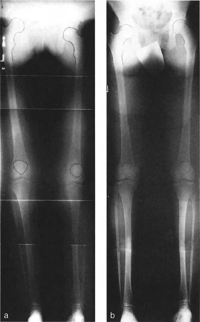
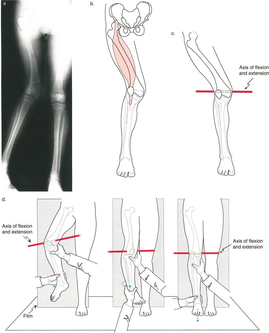
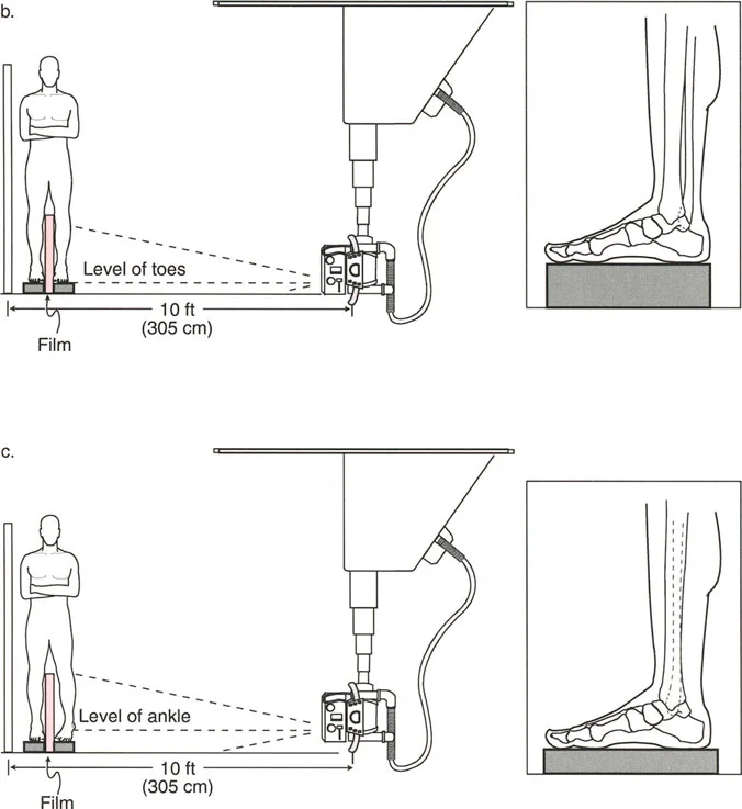
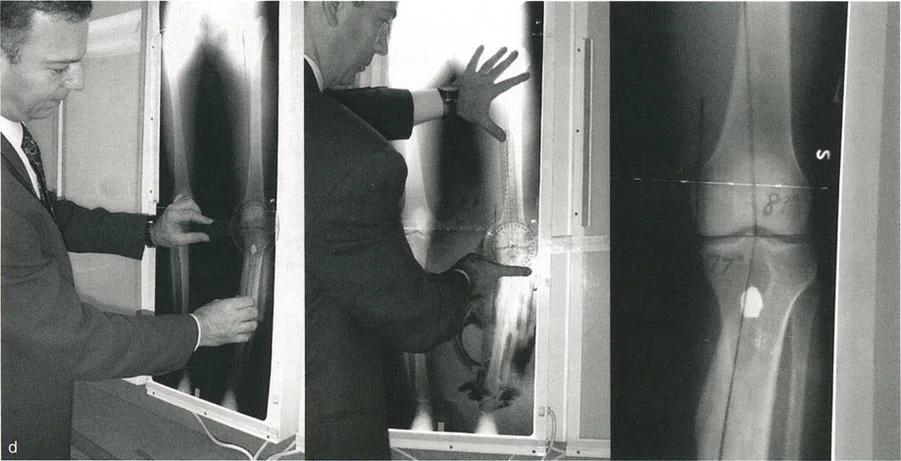
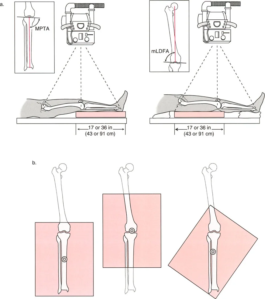
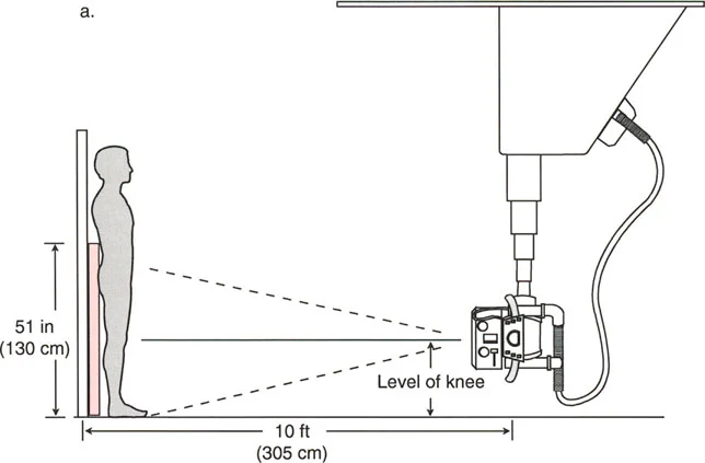
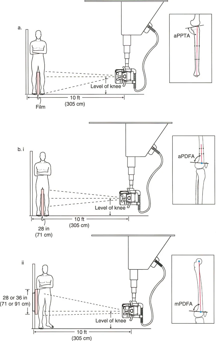
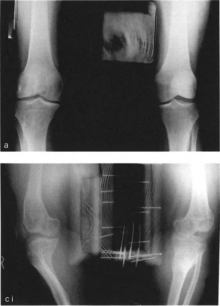
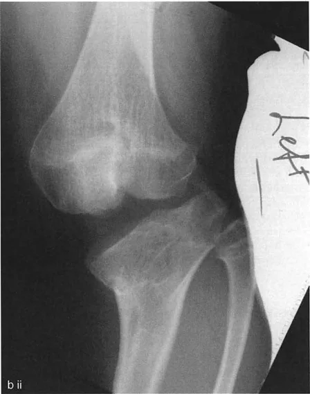
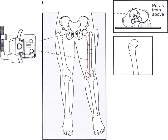
The Malalignment Test is a systematic, algorithmic radiographic evaluation designed by Dr. Paley to identify the exact anatomical sources of Mechanical Axis Deviation. It requires a high-quality, standing, full-length, weight-bearing anteroposterior radiograph of both lower extremities, with the patellae oriented strictly forward.
The Malalignment Test isolates whether the deformity originates from the femur, the tibia, the joint space itself, or a combination of these factors.
Step Zero Measuring Mechanical Axis Deviation
The foundation of the Malalignment Test begins with establishing the presence and magnitude of the deformity.
- Identify Joint Centers Mark the exact center of the femoral head using Mose concentric circles. Mark the center of the tibial plafond at the ankle. Mark the center of the knee joint, typically located at the midpoint between the tibial spines.
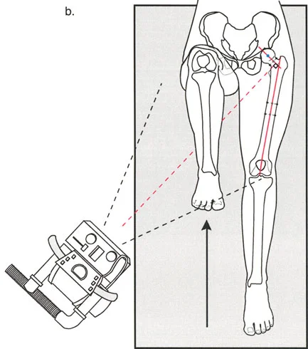
- Draw the Mechanical Axis Use a long straight edge to draw a line connecting the center of the femoral head to the center of the ankle. This is the mechanical axis of the limb.
- Measure the Deviation Mark the intersection of this mechanical axis line with the knee joint line. Measure the perpendicular distance from this intersection point to the anatomical center of the knee.
- Determine Direction Indicate whether the deviation is medial or lateral to the center of the knee.
A medial Mechanical Axis Deviation greater than 15 mm is classified as varus malalignment. A lateral Mechanical Axis Deviation of any magnitude (or medial deviation less than 1 mm) is classified as valgus malalignment.
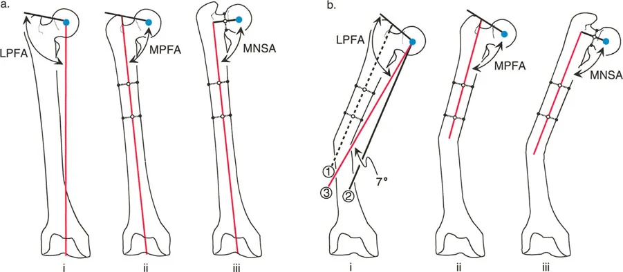
Step One Evaluating the Femur and mLDFA
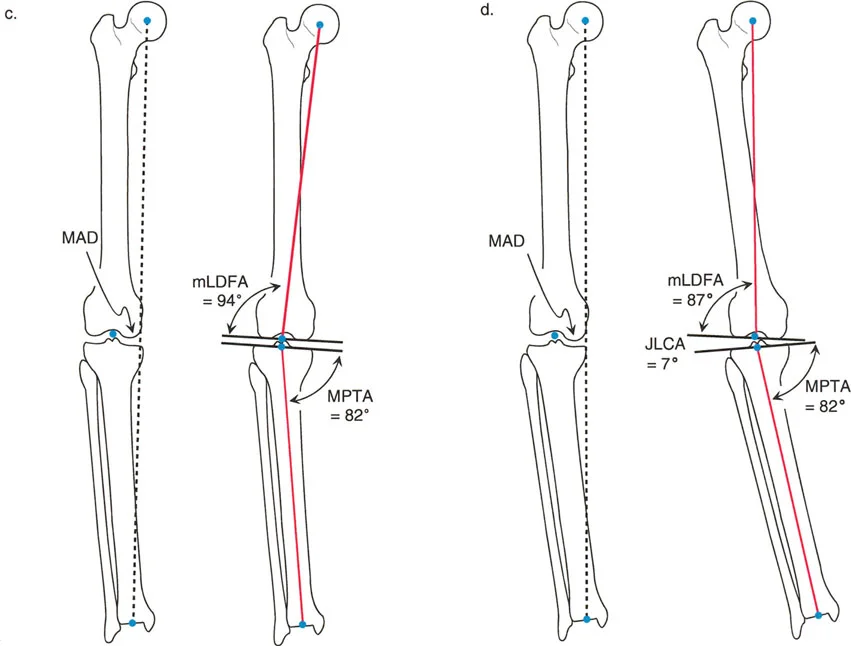
Once a pathological Mechanical Axis Deviation is confirmed, the next step is to evaluate the distal femur's contribution to the deformity. This is done by measuring the mechanical Lateral Distal Femoral Angle.
- Draw the Femoral Joint Line Draw a line tangential to the most distal points of the medial and lateral femoral condyles.
- Draw the Femoral Mechanical Axis Draw a line from the center of the femoral head to the center of the knee joint.
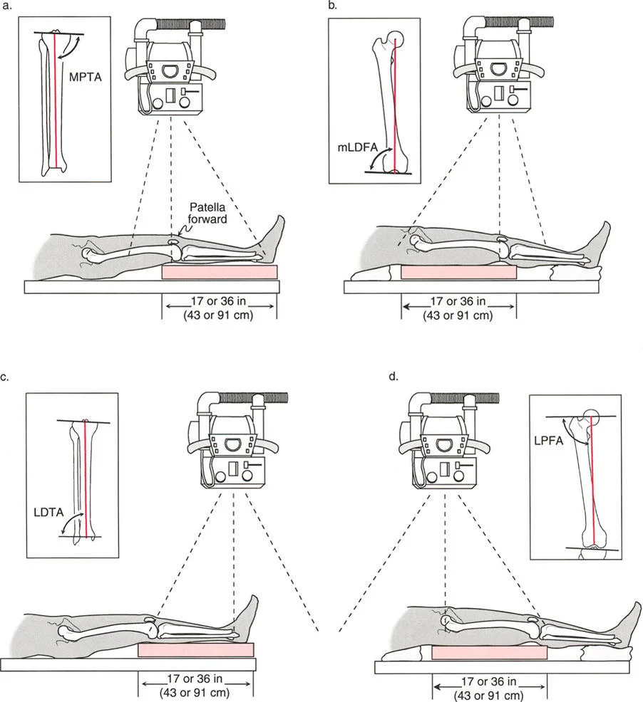
- Measure the Angle Measure the lateral angle formed by the intersection of the femoral joint line and the femoral mechanical axis.
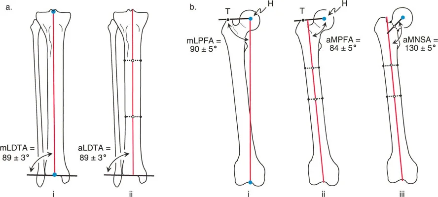
The normal range for the mechanical Lateral Distal Femoral Angle is 85 to 90 degrees.
* If the angle is greater than 90 degrees, the femur has a varus deformity contributing to medial Mechanical Axis Deviation.
* If the angle is less than 85 degrees, the femur has a valgus deformity contributing to lateral Mechanical Axis Deviation.
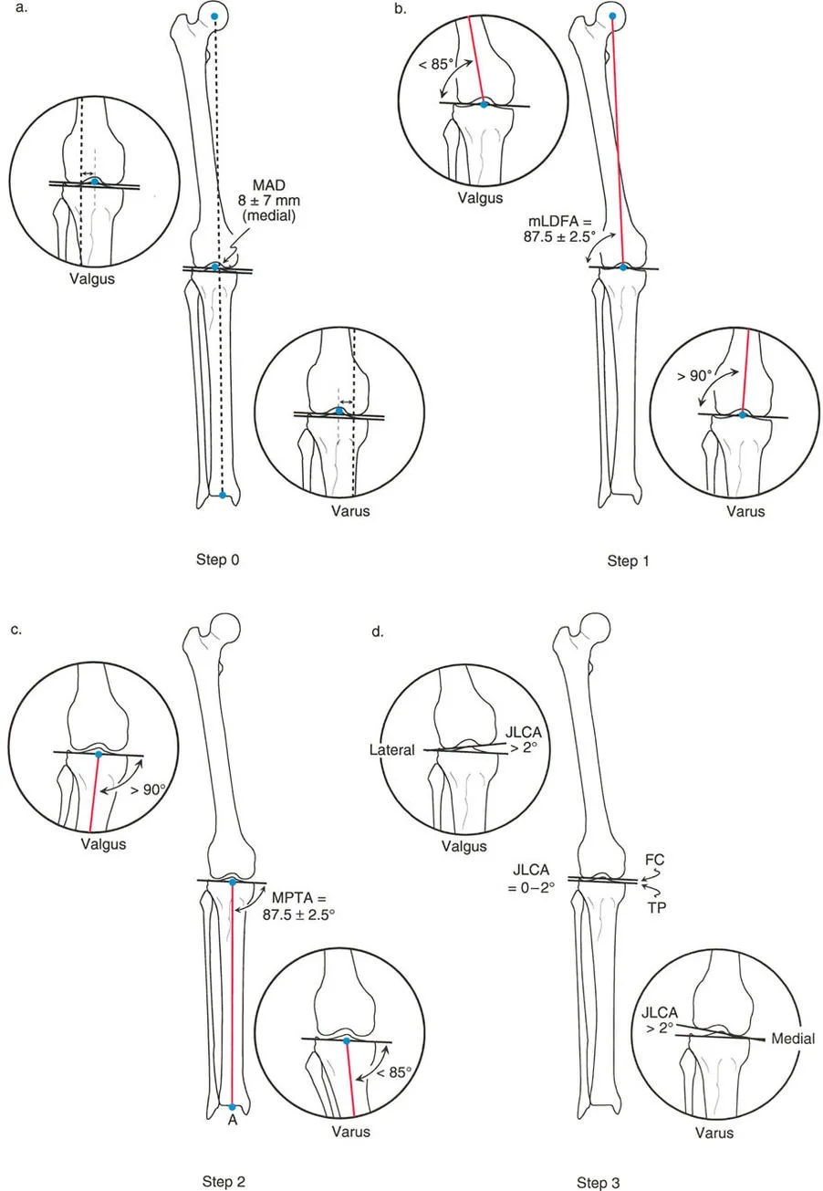
Step Two Evaluating the Tibia and MPTA
Following the femoral evaluation, the proximal tibia must be assessed using the Medial Proximal Tibial Angle.
- Draw the Tibial Joint Line Draw a line across the flat, subchondral surfaces of the medial and lateral tibial plateaus.
- Draw the Tibial Mechanical Axis Draw a line from the center of the ankle to the center of the knee joint.
- Measure the Angle Measure the medial angle formed by the intersection of the tibial joint line and the tibial mechanical axis.
The normal range for the Medial Proximal Tibial Angle is 85 to 90 degrees (average 87 degrees).
* If the angle is less than 85 degrees, the tibia has a varus deformity contributing to medial Mechanical Axis Deviation.
* If the angle is greater than 90 degrees, the tibia has a valgus deformity contributing to lateral Mechanical Axis Deviation.
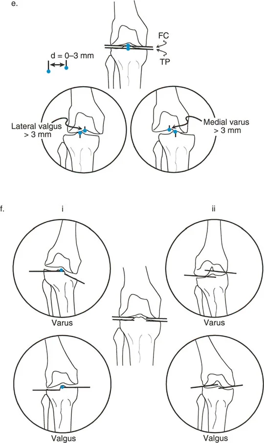
Step Three Assessing Joint Line Convergence Angle
Deformity is not always osseous; it can be driven by the soft tissues and cartilage space within the joint itself. The Joint Line Convergence Angle evaluates this interosseous contribution.
- Identify the Joint Lines Utilize the distal femoral joint line and the proximal tibial joint line drawn in the previous steps.
- Measure the Convergence Measure the angle formed between these two lines. For small angles, the Cobb method is highly effective.
- Determine Direction Note whether the lines converge medially or laterally.
Normally, the femoral and tibial joint lines are nearly parallel, exhibiting a slight medial convergence of 0 to 2 degrees.
* A medial convergence greater than 2 degrees indicates lateral ligamentous laxity or medial cartilage loss, driving medial Mechanical Axis Deviation (varus).
* A lateral convergence (lines opening medially) indicates medial ligamentous laxity or lateral cartilage loss, driving lateral Mechanical Axis Deviation (valgus).
Advanced Joint Line Analysis
Beyond the standard three steps of the Malalignment Test, Dr. Paley introduced critical addendums to rule out complex joint subluxations and condylar malorientations that can mimic or exacerbate diaphyseal deformities.
Identifying Interosseous Malalignment
Interosseous malalignment occurs when the femur and tibia themselves possess normal osseous geometry (normal mechanical Lateral Distal Femoral Angle and Medial Proximal Tibial Angle), but the relationship between them is distorted.
To evaluate for knee joint subluxation, compare the midpoints of the femoral and tibial joint lines. In a normal knee, these midpoints should be collinear within 3 mm.
* If the midpoint of the tibial joint line is translated more than 3 mm laterally relative to the femoral midpoint, this lateral subluxation is a source of lateral Mechanical Axis Deviation.
* If the midpoint is translated medially, it acts as a source of medial Mechanical Axis Deviation.
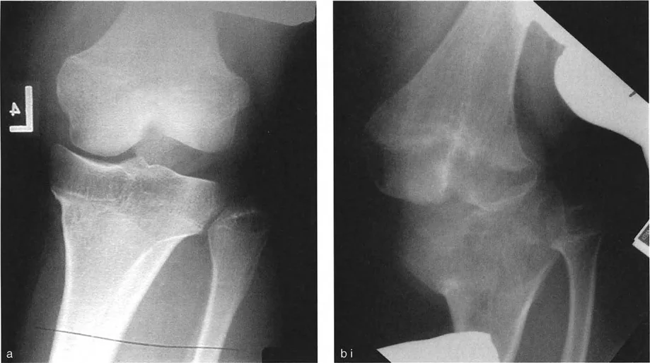
Surgeons must differentiate between joint line convergence caused by cartilage loss versus ligamentous laxity. This differentiation requires comparing weight-bearing radiographs with non-weight-bearing or stress radiographs. Ligamentous laxity will correct or alter under stress, whereas structural cartilage loss remains rigid.
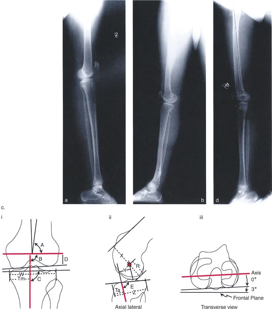
Identifying Condylar Malalignment
Condylar malalignment refers to localized intra-articular deformities where a specific condyle or plateau is depressed, hypoplastic, or maloriented, while the overall shaft of the bone remains straight.
To assess this, evaluate the collinearity of the individual plateaus and condyles:
1. Tibial Plateau Collinearity Compare the joint line of the medial plateau with the lateral plateau. They should form a single, continuous collinear line. If the medial plateau is depressed (e.g., following a medial plateau fracture malunion), it creates a localized varus source. If the lateral plateau is depressed, it creates a localized valgus source.
2. Femoral Condyle Collinearity Compare the tangent lines of the medial and lateral femoral condyles. A hypoplastic lateral femoral condyle will result in a false valgus Joint Line Convergence Angle and contribute to lateral Mechanical Axis Deviation.
Summary Table of Frontal Plane Deformity Sources
| Anatomical Source | Pathological Finding | Deformity Type | Contribution to MAD |
|---|---|---|---|
| Femur (Osseous) | mLDFA > 90° | Femoral Varus | Medial MAD |
| Femur (Osseous) | mLDFA < 85° | Femoral Valgus | Lateral MAD |
| Tibia (Osseous) | MPTA < 85° | Tibial Varus | Medial MAD |
| Tibia (Osseous) | MPTA > 90° | Tibial Valgus | Lateral MAD |
| Joint (Interosseous) | JLCA > 2° (Medial) | Cartilage loss / Laxity | Medial MAD (Varus) |
| Joint (Interosseous) | JLCA Lateral | Cartilage loss / Laxity | Lateral MAD (Valgus) |
| Joint (Subluxation) | Tibial shift > 3mm Medial | Medial Subluxation | Medial MAD |
| Joint (Subluxation) | Tibial shift > 3mm Lateral | Lateral Subluxation | Lateral MAD |
Paley Center of Rotation of Angulation Principles
Identifying the source of the deformity is only the first half of the surgical equation. The second half involves determining exactly where and how to cut the bone to correct the deformity without inducing secondary translation. This is governed by Paley's Center of Rotation of Angulation (CORA) principles.
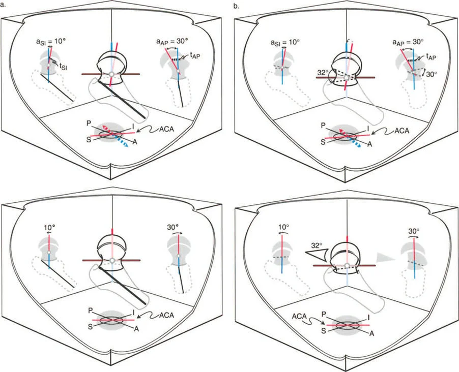
Defining the CORA
The Center of Rotation of Angulation represents the exact point where the proximal mechanical axis line and the distal mechanical axis line of a deformed bone intersect.
To find the CORA:
1. Draw the normal mechanical (or anatomic) axis line of the proximal bone segment.
2. Draw the normal mechanical (or anatomic) axis line of the distal bone segment.
3. The intersection of these two lines is the CORA. The angle formed between them is the true magnitude of the angular deformity.
A single bone may have a uniapical deformity (one CORA) or a multiapical deformity (multiple CORAs). Accurately mapping the CORA is non-negotiable for precise surgical planning.
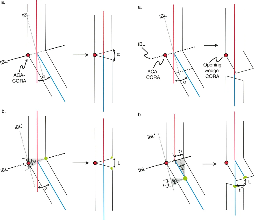
The Three Osteotomy Rules
Dr. Paley formulated three fundamental osteotomy rules that dictate the geometric outcome of a bone cut relative to the CORA and the Axis of Correction of Angulation (ACA). The ACA is the physical hinge point around which the bone fragments are rotated during surgery.
Osteotomy Rule 1: Pure Angulation
When the osteotomy line and the Axis of Correction of Angulation both pass directly through the CORA, the result is pure angular correction. The bone ends will angulate without any translation, resulting in perfect realignment of the mechanical axis. This is the ideal scenario for most deformity corrections.
Osteotomy Rule 2: Angulation with Planned Translation
When the Axis of Correction of Angulation passes through the CORA, but the osteotomy is performed at a different level (above or below the CORA), the bone will undergo angular correction accompanied by a predictable, obligatory translation of the bone ends.
* Clinical Pearl: This rule is frequently utilized when the CORA is located very close to a joint line where poor bone stock exists. The surgeon places the hinge (ACA) at the joint line CORA but makes the actual bone cut (osteotomy) further down the metaphysis or diaphysis to ensure better healing and fixation, accepting the resulting translation.
Osteotomy Rule 3: Creation of Translation Deformity
If the osteotomy and the Axis of Correction of Angulation are placed at a level independent of the CORA, the correction of the angle will result in a secondary translation deformity. The mechanical axis will remain misaligned, presenting as a parallel shift (zigzag deformity). This is considered a surgical error unless intentionally used to correct a pre-existing translational deformity.
Comprehensive Preoperative Planning
Successful execution of Paley's principles requires meticulous preoperative planning. The surgeon must transition from the radiographic analysis to a tangible surgical blueprint.
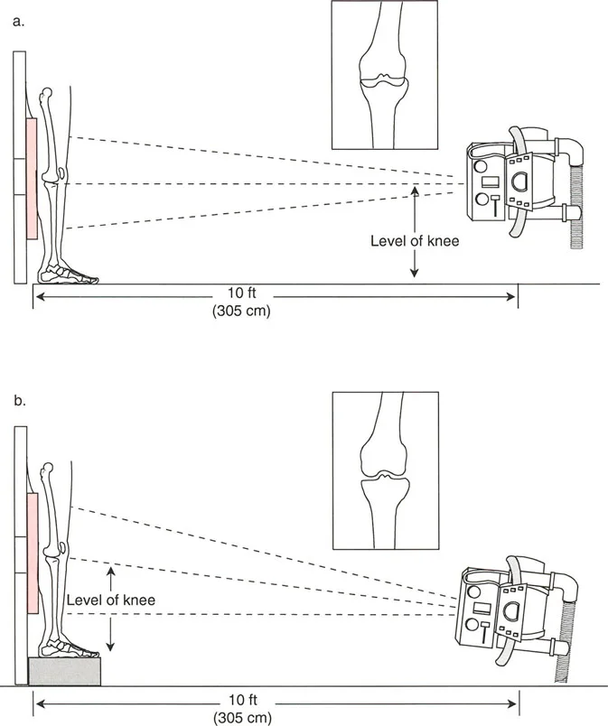
Radiographic Requirements
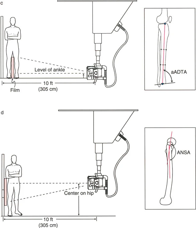
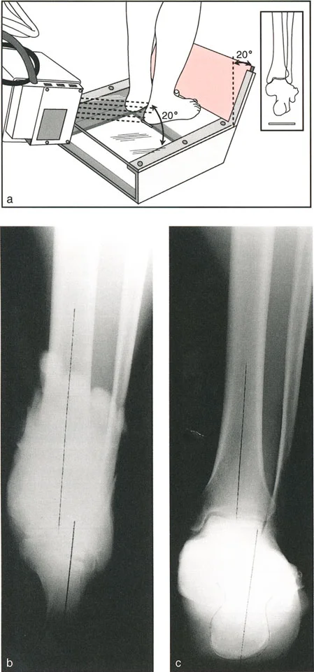
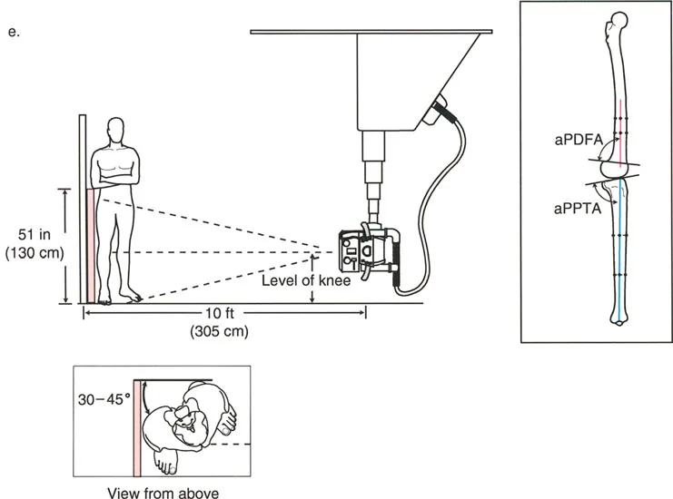
Standardizing the imaging protocol is vital. A slight rotation of the limb can drastically alter the projected joint angles, leading to erroneous measurements.
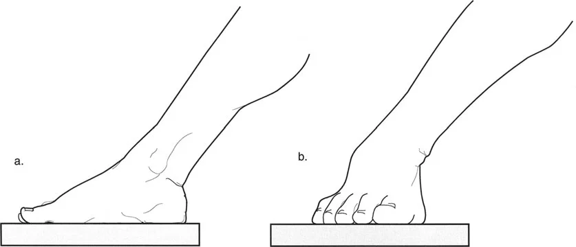
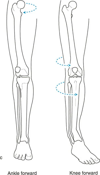
* Patellar Orientation: The patella must be facing strictly forward, regardless of foot position. This isolates the frontal plane deformity from any rotational malalignment.
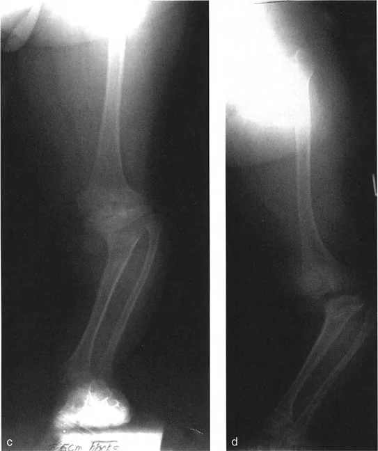
* Magnification Markers: Radiographs must include a scaling marker (typically a 25 mm spherical marker) to allow for accurate digital templating and measurement of leg length discrepancies.
* Weight-Bearing Status: Films must be weight-bearing to accurately assess the dynamic Joint Line Convergence Angle and true Mechanical Axis Deviation under physiological load.
Systematic Deformity Analysis
When approaching a complex lower extremity deformity, the surgeon should follow a strict checklist:
- Assess Leg Length Discrepancy: Measure the absolute lengths of the femur and tibia bilaterally.
- Perform the Malalignment Test: Execute Steps 0 through 3 to map the Mechanical Axis Deviation, mechanical Lateral Distal Femoral Angle, Medial Proximal Tibial Angle, and Joint Line Convergence Angle.
- Identify the Primary Source: Determine if the primary driver of the deformity is osseous (femur/tibia), interosseous (joint laxity), or condylar.
- Locate the CORA: Draw the proximal and distal mechanical axes of the deformed bone segment to find the apex of the deformity.
- Select the Osteotomy Rule: Decide whether a Rule 1, Rule 2, or Rule 3 osteotomy is clinically appropriate based on soft tissue envelopes, bone quality, and fixation methods.
- Plan the Fixation: Choose between internal fixation (plates/nails) for acute correction or external fixation (circular frames/hexapod systems) for gradual correction.
Surgical Pearls for Frontal Plane Correction
- Addressing the Fibula: In proximal tibial osteotomies for varus/valgus correction, the fibula often acts as a lateral tether. A fibular osteotomy or proximal tibiofibular joint release is frequently necessary to achieve full correction without excessive force.
- Managing the Peroneal Nerve: Large valgus corrections (e.g., closing wedge distal femoral osteotomies or opening wedge proximal tibial osteotomies) can stretch the common peroneal nerve. Prophylactic peroneal nerve decompression should be considered for acute corrections exceeding 10 to 12 degrees.
- Hinge Placement: When performing an opening wedge osteotomy, the hinge (ACA) must be placed precisely at the convex cortex (the CORA). If the hinge is placed too far inward, the bone will translate. If the hinge cortical bridge breaks, stability is lost, and unwanted translation may occur.
- Soft Tissue Balancing: Remember that osseous correction alone will not resolve a high Joint Line Convergence Angle driven by ligamentous laxity. In severe cases, concurrent soft tissue reconstruction (e.g., collateral ligament advancement) or over-correction of the mechanical axis may be required to unload the deficient compartment.
By strictly adhering to the Malalignment Test and Paley's CORA principles, orthopedic surgeons can deconstruct even the most complex frontal plane deformities into manageable, geometric components. This systematic approach ensures highly predictable surgical outcomes, restores optimal joint biomechanics, and significantly enhances patient longevity and function.
!!! info "Academic Resource & Medical Review"
This academic resource was prepared and medically reviewed by Prof. Dr. Mohammed Hutaif, Consultant Orthopedic & Spine Surgeon. It is formulated specifically for medical students, orthopedic residents, and surgeons preparing for high-stakes board examinations (AAOS, FRCS Tr & Orth, Arab Board).
!!! warning "Disclaimer"
The surgical techniques, classifications, and clinical guidelines presented herein are for educational and academic review purposes only. They are not intended to replace institutional protocols or independent clinical judgment.
You Might Also Like